The big statistical question of what is regression analysis. Dive into statistics with this article about regression analysis.
Table of Contents:
Regression Analysis
Regression analysis is one of the most widely used statistical techniques, particularly in fields such as economics, finance, healthcare, and engineering. It allows us to understand the relationships between different variables and predict outcomes based on input data. Whether you want to model the relationship between a country’s GDP and its employment rate, or predict housing prices based on features like size and location, regression analysis provides a powerful and flexible framework.
In this content, we’ll explore into the key types of regression analysis, explain the steps involved in conducting a regression, discuss important assumptions to check, and highlight its wide-ranging applications.
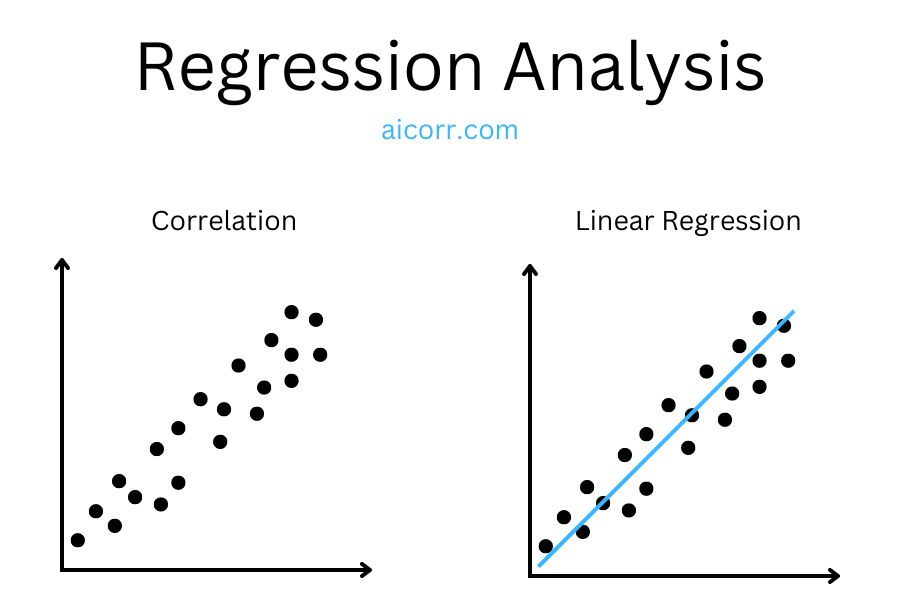
What is Regression Analysis?
Regression analysis is essentially a way to estimate the relationships among variables. At its core, the goal is to predict the dependent variable (also known as the response or outcome variable) based on one or more independent variables (also known as predictors or explanatory variables).
The simplest form of regression is a linear relationship, which assumes that the change in the dependent variable is proportional to the change in the independent variable(s). However, regression analysis can take many forms, extending to more complex relationships, such as polynomial or logistic models.

Types of Regression Analysis
Regression analysis comes in different forms, depending on the nature of the data and the relationships among variables. The following are the most common types.
1. Simple Linear Regression
Simple linear regression examines the relationship between two variables: one independent and one dependent. It assumes that the relationship between the variables can be expressed as a straight line, using the following equation:

Here, y represents the dependent variable, x is the independent variable, β0 is the intercept, and β1 is the slope of the line. The term ϵ represents the error term, accounting for the variation in y that isn’t explained by x.
For example, simple linear regression might be used to model the relationship between a person’s height (independent variable) and their weight (dependent variable). In such a case, the slope of the line β1 tells us how much a change in height affects weight.
2. Multiple Linear Regression
In real-world scenarios, outcomes are often influenced by more than one factor. Multiple linear regression extends the concept of simple linear regression to include multiple independent variables. The general form of the equation becomes:

y = β0 + β1×1 + β2×2 + … + βnxn + ϵ
Each xi represents an independent variable, and each βi coefficient shows how much that variable affects the outcome y, holding all other variables constant.
For instance, in predicting house prices, we may use several predictors such as the size of the house, number of bedrooms, location, and age of the property. Multiple linear regression allows us to understand how each factor contributes to the final price.
3. Logistic Regression
Not all outcomes are continuous. Logistic regression is used when the dependent variable is categorical, often binary. Rather than predicting a continuous outcome, logistic regression predicts the probability of a particular event occurring. The relationship between the predictors and the probability is modelled through a logistic function, which produces results between 0 and 1:

Logistic regression is widely used in classification problems. For example, it can predict whether a customer will purchase a product (yes/no) based on factors like income, age, and browsing behavior.
4. Polynomial Regression
In many cases, the relationship between variables may not be linear. Polynomial regression is a type of regression that models the relationship as an nth-degree polynomial. For example, the model could look like:

This type of regression is useful for modeling more complex, curved relationships. For instance, polynomial regression could apply to model population growth, which may accelerate at a rate faster than a straight line can represent.
5. Ridge and Lasso Regression (Regularisation Techniques)
When working with multiple predictors, the problem of multicollinearity can arise, where independent variables are highly correlated with each other, leading to unstable coefficient estimates. To address this, ridge regression and lasso regression apply regularisation techniques, adding a penalty to the size of the coefficients:
- Ridge Regression: Adds a penalty based on the sum of squared coefficients, shrinking large coefficients and preventing overfitting.
- Lasso Regression: Similar to ridge but can shrink some coefficients to exactly zero, effectively performing variable selection and removing irrelevant predictors from the model.
Steps in Conducting Regression Analysis
Conducting a regression analysis involves several steps.
1. Data Collection
The first step is collecting relevant data on the dependent and independent variables. The quality and quantity of the data are crucial for the success of the regression model.
2. Model Fitting
Once the data is collected, the next step is to fit a regression model using statistical software such as Python (via statsmodels or scikit-learn), R, or Excel. This involves estimating the coefficients β0, β1, …, βn that best describe the relationship between the variables.
3. Interpreting Coefficients
After fitting the model, you can interpret the estimated coefficients. In simple linear regression, β1 tells us how much the dependent variable changes for each unit change in the independent variable. In multiple regression, each coefficient shows the effect of one predictor while holding others constant.
4. Checking Assumptions
Before trusting the model’s results, it’s important to check the following assumptions:
- Linearity: The relationship between predictors and the outcome should be linear.
- Independence: The observations should be independent of each other.
- Homoscedasticity: The variance of the errors should be constant across all levels of the independent variables.
- Normality: The residuals should be normally distributed.
5. Model Evaluation
The most common way to evaluate a regression model is by looking at the R-squared (R²) value, which represents the proportion of variance in the dependent variable explained by the model. Higher R² values indicate better model fit. Adjusted R² is a more conservative version of this metric, adjusting for the number of predictors in the model.
6. Prediction
Once the model is validated, it can be used to predict outcomes for new data points. For example, a real estate company might use the model to predict the price of a house that hasn’t been sold yet.
Applications of Regression Analysis
Regression analysis is applies across a wide range of industries.
- Economics and Finance: To predict GDP growth, stock prices, or inflation rates.
- Healthcare: To identify risk factors for diseases, or predict patient outcomes based on treatment.
- Marketing: To estimate customer demand, optimise pricing strategies, and predict consumer behavior.
- Engineering: To model complex systems and predict outcomes such as energy consumption, material wear, or system failures.
The Bottom Line
Regression analysis is an indispensable tool for understanding relationships between variables and making predictions based on data. Whether you’re working with simple or complex data, this technique provides a rigorous framework for analysing patterns and making data-driven decisions. By choosing the right type of regression, checking assumptions, and interpreting results carefully, you can extract valuable insights that drive informed actions across various fields.